
Ripley’s K and Besag’s L Function
Published:
Summary: This note introduces Ripley’s $K$ and Besag’s $L$ functions for analyzing spatial point patterns. It explains CSR as the null model, defines and estimates $K(r)$ with edge corrections, variance-stabilization via $L(r)$, and the need for Monte Carlo envelopes. Redwood data illustrate clustering versus intensity-driven inhomogeneity.
1. Motivation
1.1 What problem are we solving?
In spatial point pattern analysis, examining the distances between events provides key insights into how those events are arranged in space. But this brings us the question:
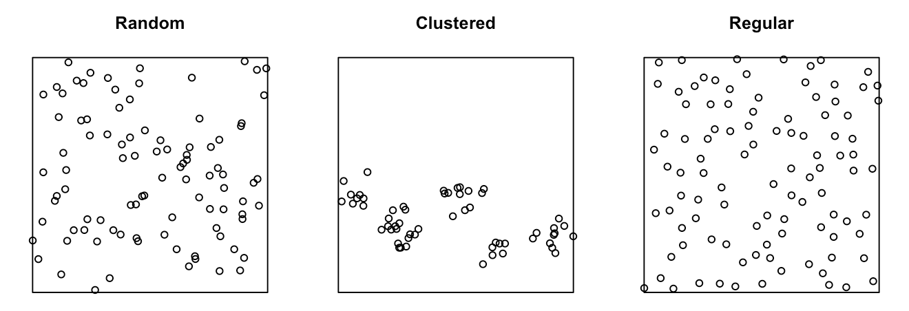
How can we tell if events (like trees, disease cases, or shops) are randomly scattered, clustered, or evenly spaced?
To measure the level of clustering, we can think of
- Setting a radius for each point and drawing a circle
- Counting neighbors within circle
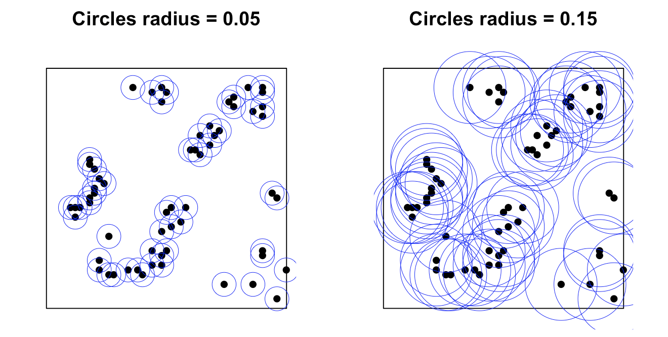
The perceived clustering pattern of the same dataset can change depending on the chosen buffer size, as spatial correlation among nearby points strongly influences the results. To quantify this relationship between spatial event patterns and distance, spatial summary statistics such as Ripley’s $K$ function and its variance-stabilized form, Besag’s $L$ function, are commonly used. These functions provide a systematic way to evaluate clustering or dispersion across different spatial scales.
1.2 Mathematical Setup
In general, we are studying a spatial point process $X = {x_1,x_2,\cdots,x_n}$ inside a finite observation window $W\subset\mathbb{R}^2$.
For example:
- $x_i=$ coordinates of events (e.g., forest fires, road accidents and etc.)
- $W=$ study region (e.g., Singapore boundary, forest plot, etc.)
- $n=$ observed number of points.
- $d_{ij}=$ Euclidean distance between $x_i$ and $x_j$.
- $r=$ radius or distance scale of buffer.
Below is a table of notations we gonna use in the following introduction:
| Symbol | Meaning | Units |
|---|---|---|
| $W$ | Observation window (bounded region) | km$^2$ |
| $x_i$ | Location of $i$-th observed point | $(x,y)$coords |
| $n$ | Number of observed points | counts |
| $d_{ij}$ | Euclidean distance between $x_i$ and $x_j$ | km |
| $r$ | Radius or distance scale | km |
| $\lambda$ | Intensity $=$ expected number of points per unit area | points/km$^2$ |
| $\hat{\lambda}$ | Empirical estimate of $\lambda$: $\hat{\lambda}=\frac{n}{|W|}$ | points/km$^2$ |
| $b(x,r)$ | Fraction of the circle of radius $r$ around $x$ inside $W$ (isotropic edge correction) | unitless |
| $w_{ij}$ | Edge-correction weight for pair $(i,j)$ | unitless |
| B | Number of Monte Carlo replicates under $\text{H}_0$ | unitless |
2.1 Null Model
Recall that our goal is to understand the relationship between spatial event patterns and distance. By introducing appropriate metrics, we can quantify this relationship; however, conclusions about “clustering” or “inhibition” are inherently inferential. To make such claims, we must compare the observed pattern against what we would expect under a scenario with no spatial structure, where events are randomly and independently distributed. This requires specifying a null model, typically based on complete spatial randomness (CSR), to serve as the benchmark for comparison.
Here, note that Complete Spatial Randomness (CSR) $=$ homogeneous Poisson process:
- Homogeneity: constant intensity $\lambda$ everywhere.
- Independence: no interaction between points.
- Probability of observing $k$ points (events) in area $A$:
Therefore, the null hypothesis would be:
\[\text{H}_0:\, \text{Points follow an homogeneous Poisson Process with constant intensity}\, \lambda\]Under CSR, the expected number of neighbors within radius $r$ of a random point is:
\[\mathbb{E}\left[\text{number of neighbors within radius}\,r\mid \text{H}_0\right] =\lambda \cdot \pi r^2.\]2.2 Ripley’s $K$ Function
2.2.1 Definition
For a stationary and isotropic point process, Ripley’s $K$ is defined as:
\[K(r) = \frac{\mathbb{E}[\text{number of other points within distance}\,r\,\text{of a typical point}]}{\lambda}\triangleq\frac{\mathbb{E}\left[ N_0(r)\right]}{\lambda}.\]where:
- $N_0(r)=$ number of other points within distance $r$ of a typical point.
- $\lambda=$ intensity.
Intuition:
Given a typical point, what’s the expected number neighbors within distance $r$, normalized by overall density?
Then under CSR, the expected number of neighbors in a circle of radius $r$ is $\lambda\pi r^2$, then we plug into the definition:
\[K_{\text{CSR}}(r)=\frac{\lambda\pi r^2}{\lambda}=\pi r^2.\]Therefore, considering that the empirical estimate of $\lambda$ is $\frac{n}{|W|}$, the Ripley’s $K$ can be approximately written as:
\[K(r)\approx \frac{\mathbb{E}\left[ N_0(r)\right]}{\hat{\lambda}}=\frac{\mathbb{E}\left[ N_0(r)\right]}{n}\cdot W.\]Since $\frac{\mathbb{E}\left[ N_0(r)\right]}{n}$ is a proportion, another interpretation of $K(r)$ is that it represents the expected area within distance r around a randomly chosen event occupied by other events, assuming the process has constant intensity.
Therefore, comparing to benchmark, we have
- $K(r)>\pi r^2\rightarrow$ more neighbors than CSR $\rightarrow$ clustering at scale $r$.
- $K(r)\approx \pi r^2 \rightarrow$ like CSR.
- $K(r)<\pi r^2\rightarrow$ fewer neighbors $\rightarrow$ regularity / inhibition.
2.2.2 Estimation
So in practice of estimating $K(r)$, to align with the theory, we must consider
- Count neighbors,
- Fix edge bias, i.e., those points near the boundary have part of their circle cut off.
A common estimator with edge correction:
\[\hat{K}(r)=\frac{|W|}{n(n-1)}\sum_{i\neq j}\frac{\mathbb{1}_{\{||x_i-x_j||\leq r\}}}{w_{ij}},\]- $\mathbb{1}_{{…}}$ is an indicator function.
- $w_{ij}$ is an edge correction weight ($\approx$ fraction of the circle around $x_i$ at radius $||x_i-x_j||$ that lies inside $W$).
- popular choices: translation, isotropic, border corrections.
note the prefactor $\frac{|W|}{n(n-1)}=\frac{1}{n\cdot \hat{\lambda}}$ under $\hat{\lambda}=\frac{n}{|W|}$.
2.2.3 Reasoning of edge correction
Basically, without correction, those points near the boundary will lose a lot of neighbors when $r$ is large, this will lead to a downward bias in $\hat{K}(r)$ due to the limitation of the study region $W$.
Thus, to address this issue, the intuition is to compensate for missing neighbor area, meaning giving higher weights to those points close to boundary. So we can use isotropic edge correction as an example.
So in isotropic edge correction, we weight each neighbor by:
\[w_{ij}=b(x_i,d_{ij})\in (0,1]\]where $b(x_i,d_{ij})=$ proportion of the circle of the circle of radius $d_{ij}$ around $x_j$ that lies inside $W$. The estimator with edge correction incorporated can be written as:
\[\hat{K}(r)=\frac{|W|}{n(n-1)}\sum_{i\neq j}\frac{\mathbb{1}_{\{||x_i-x_j||\leq r\}}}{b(x_i,d_{ij})}\]- If the circle is fully inside, $b=1 \rightarrow$ no correction,
- if half the circle is inside, $b=0.5\rightarrow$ double the weight.
2.2.4 Practical Workflow for Ripley’s $K$ function
Choose a set of radius $r_1,\cdots,r_m$ (e.g., a grid from small to large distances, not exceeding the window’s border). Pragmatically, can use \(r_{max}\approx \min(\text{window\_width},\text{window\_length})/4.\)
- Compute $\hat{K}(r_k)$ (with edge correction).
- Generate Monte Carlo envelopes under $\text{H}_0$:
- Simulate $B$ Monte Carlo replicates under $\text{H}_0$ in $W$ with intensity $\hat{\lambda}$,
- For each $r_k$, we collect ${\hat{K}^{*(b)}(r_k)}_{b=1}^{B}$,
- Take the empirical $2.5$% and $97.5$% percentiles as a pointwise $95$% envelope,
- Compare the observed curve with the envelope:
- Observed $\hat{K}(r_k)$ above envelope $\rightarrow$ significant clustering at those $r_k$,
- Observed $\hat{K}(r_k)$ below envelope $\rightarrow$ significant inhibition.
2.3 Besag’s $L$ Function
2.3.1 Definition
The variance of $\hat{K}(r)$ increases quadratically with r, since under CSR, recall that \(K_{\text{CSR}}(r)=\pi r^2\)So to stabilize variance and also to make the curve more visually comparable across $r$, Besag (1977) defined the $L$ function:
\[L(r)=\sqrt{\frac{K(r)}{\pi}}\]Then under CSR:
\[L_{CSR}(r)=r\]For better visual interpretation, some may also plot the centered $L$ function:
\[L(r)-r\]so CSR sits at 0:
- $L(r)-r>0 \rightarrow$ clustering at distance $r$,
- $L(r)-r\approx 0 \rightarrow$: CSR-like,
- $L(r)-r<0\rightarrow$ inhibition.
2.2.4 Practical Workflow for Besag’s $L$ function
Choose a set of radius $r_1,\cdots,r_m$ (e.g., a grid from small to large distances, not exceeding the window’s border). Pragmatically, can use \(r_{max}\approx \min(\text{window\_width},\text{window\_length})/4.\)
- Compute $\hat{K}(r_k)$ (with edge correction), then $\hat{L}(r_k)-r_k$.
- Generate Monte Carlo envelopes under $\text{H}_0$:
- Simulate $B$ Monte Carlo replicates under $\text{H}_0$ in $W$ with intensity $\hat{\lambda}$,
- For each $r_k$, we collect ${\hat{L}^{*(b)}(r_k)-r_k}_{b=1}^{B}$,
- Take the empirical $2.5$% and $97.5$% percentiles as a pointwise $95$% envelope,
- Compare the observed curve with the envelope:
- Above envelope $\rightarrow$ significant clustering at those $r$;
- Below envelope $\rightarrow$ significant inhibition.
3. Inhomogeneity vs. Independence
When observing $\hat{K}(r)$ significantly deviates from the null hypothesis $\text{H}_0$’s expectation $\pi r^2$, then you have certainly have evidence to reject $\text{H}_0$ at those scales. However, we should note that rejecting $\text{H}_0$ doesn’t automatically mean clustering or inhibition.
For example, when observing $\hat{K}(r)\gg \pi r^2$, it suggests “apparent” clustering at that $r$, whilst “apparent” doesn’t equal to “true”. As the violation of $\text{H}_0$ might come from:
- Inhomogeneous intensity $\lambda(x)$ varies across $x$, where $x \subset W$. This could be caused by population density, environmental covariates, like residents in rural area tend to have sparse population density, therefore the incident disease cases are far fewer than that in urban area.
- True inter-point interaction (dependence), which is our real focus of interest.
Hence, when having some prior knowledge or observing $\hat{K}(r)\neq \pi r^2$, to eliminate possible confounders like Inhomogeneity, we should consider a new null hypothesis:
\[\text{H}_0:\, \text{Points follow an inhomogeneous Poisson Process with intensity}\, \lambda(x)\]This means that intensity can vary by regions but points are independent given $\lambda(x)$.
And under the new $\text{H}_0$, we adjust the estimator like this:
\[\hat{K}_\text{inhom}(r)=\frac{1}{|W|}\sum_{i\neq j}\frac{\mathbb{1}_{d_{ij}\leq r}}{\hat{\lambda}(x_i)\hat{\lambda}(x_j)}\cdot \frac{1}{w_{ij}}\]4. Reasoning of Monte Carlo Simulation (Require further explanation)
Since the theoretical expectation of Ripley’s $K(r)$ is fixed at $\pi r^2$, so shouldn’t we be able to analytically derive confidence intervals for $\hat{K}(r)$ without sampling? Why do we need Monte Carlo envelopes at all?
Certainly there are some analytic approaches, but their limitations greatly make the calculation and implementation much more complicated:
- They all assume large $n$
- They all assume rectangle or infinite $W$ (e.g., no border)
- $Var(\hat{K}(r))$ isn’t simply the variance of a binomial proportion, as local clustering causes covariance between pairs and points share neighbors, making the analytical form extremely hard to be derived in practice.
5. Real-world Example
In this section, we will calculate Ripley’s $K$ and Besag’s $L$ on redwood dataset in spatstat package in R to better understand the theory.
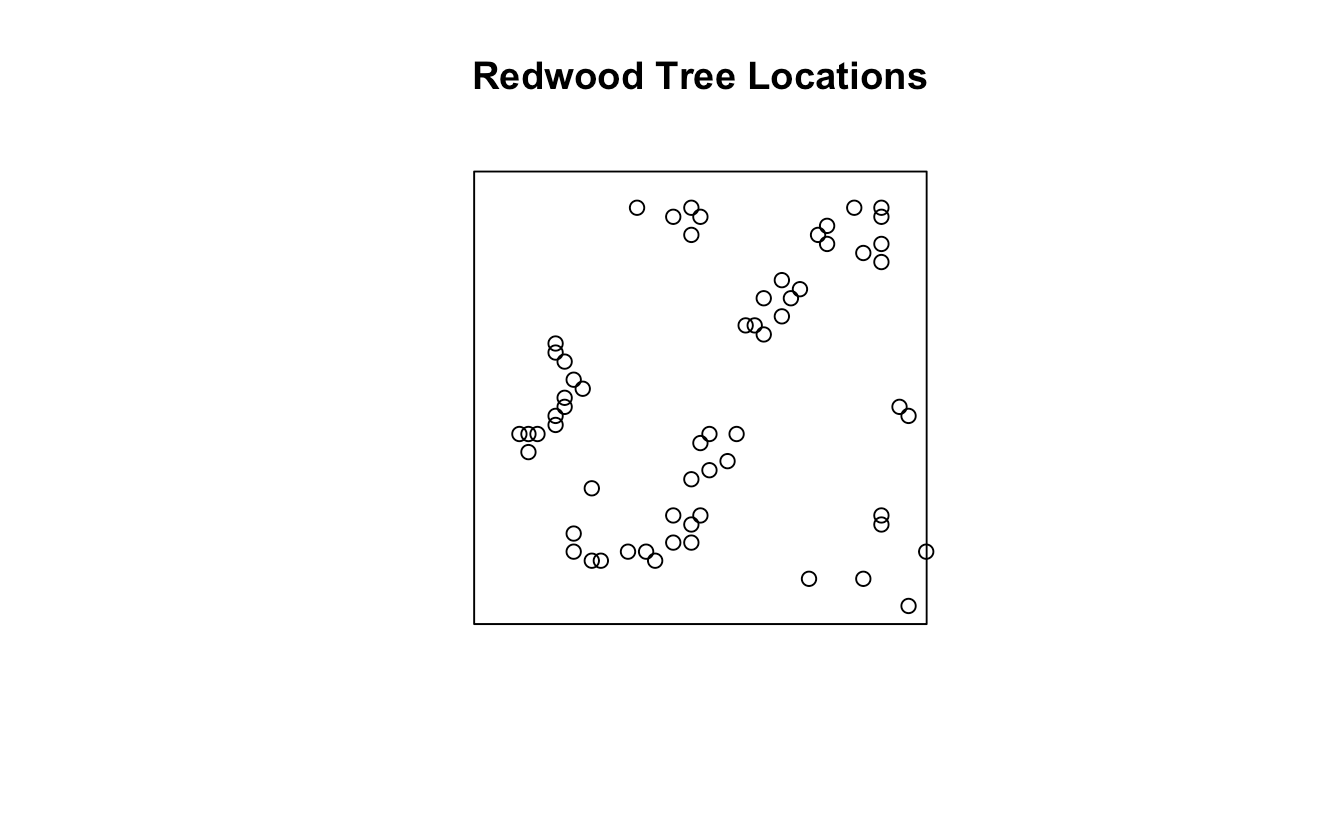
The redwood dataset represents the spatial locations of 195 redwood trees in a unit square region. Each tree has an $(x,y)$ coordinate within the square $[0,1]\times [0,1]$. And the data were simulated to mimic clustering typical of natural forests, based on a Neyman-Scott cluster process.
We first set up the environment, load all required packages and dataset into the environment. Then we can draw the plot to see the study region and spatial distribution of events in following figure.
# ---------- 0) Setup ----------
pkgs <- c("spatstat.data", "spatstat.geom", "spatstat.explore", "spatstat.random")
to_install <- pkgs[!sapply(pkgs, requireNamespace, quietly = TRUE)]
if (length(to_install)) install.packages(to_install, repos = "https://cloud.r-project.org")
lapply(pkgs, library, character.only = TRUE)

# ---------- 1) Load redwood tree dataset ----------
data("redwood", package = "spatstat.data")
X <- redwood
plot(X, main = "Redwood Tree Locations")
And then we choose use up to $1/4$ of the smaller window side length to avoid strong edge effects as the analysis range of $r$.
# ---------- 2) Choose analysis range r ----------
win <- Window(X)
side_min <- min(diff(as.vector(win$xrange)), diff(as.vector(win$yrange)))
rmax <- side_min / 4
rvals <- seq(0, rmax, length.out = 128)
After everything ready, we move on to compute Ripley’s $K$ across selected $r$. Note that here for simplicity, we still assume the $\text{H}0$ is under Poisson process, which means the CSR benchmark is $K{CSR}(r)=\pi r^2$. And we use isotropic edge correction in this case.
# ---------- 3) K-function (CSR benchmark: K_theo = pi r^2) ----------
# Compute K with isotropic edge correction (plus border for reference).
K <- Kest(X, r = rvals, correction = c("isotropic", "border"))
# Monte Carlo envelope under CSR (same window, Poisson with same intensity)
set.seed(123)
envK <- envelope(X, fun = Kest, nsim = 199, r = rvals,
                 correction = "isotropic", global = FALSE, savefuns = TRUE)

# Plot K with CSR envelope
plot(envK, . ~ r, main = "Ripley's K with CSR envelope (isotropic correction)",
     legend = FALSE)
.png) Clearly, this plot shows Ripley’s $K(r)$ (black) versus the CSR expectation $\pi r^2$ (red) with a $95$% Monte Carlo envelope (gray). Since the observed $K(r)$ lies mostly above the envelope for small to medium distances, the pattern displays significant clustering at these spatial scales compared to complete spatial randomness.
Clearly, this plot shows Ripley’s $K(r)$ (black) versus the CSR expectation $\pi r^2$ (red) with a $95$% Monte Carlo envelope (gray). Since the observed $K(r)$ lies mostly above the envelope for small to medium distances, the pattern displays significant clustering at these spatial scales compared to complete spatial randomness.
Then similarly, we further compute Besag’s $L$:
# ---------- 4) L-function ----------
# L(r) = sqrt(K(r)/pi). 'Lest' directly estimates L; the theoretical line is L_theo = r.
L <- Lest(X, r = rvals, correction = "isotropic")

# Also compute envelope for L (by transforming the stored K simulations)
# Simpler: build envelopes directly on Lest
set.seed(123)
envL <- envelope(X, fun = Lest, nsim = 199, r = rvals,
                 correction = "isotropic", global = FALSE)
# Plot L with CSR envelope; add L=r reference
plot(envL, . ~ r, main = "Besag's L with CSR envelope (isotropic correction)",
     legend = FALSE)
abline(0, 1, lty = 2)
.png) This plot almost suggests the same conclusion that the point pattern exhibits clustering starting from $0.04-0.18$.
This plot almost suggests the same conclusion that the point pattern exhibits clustering starting from $0.04-0.18$.
We also draw the centered Besag’s $L$ with CSR envelope to better visually interpret:
envL_centered <- envL
envL_centered$obs <- envL$obs - envL$r
envL_centered$lo <- envL$lo - envL$r
envL_centered$hi <- envL$hi - envL$r
envL_centered$theo <- 0
# Plot L with CSR envelope; add L=r reference
plot(envL_centered, . ~ r, main = "Centered Besag's L with CSR envelope (isotropic correction)",
     legend = FALSE)
abline(0, 1, lty = 2)
.png)
So now we have observed great violation of $\text{H}_0$, so to eliminate the potential confounding of varying $\lambda(x)$ across different regions, we need to use inhomogeneous Poisson process:
# ---------- 5) Inhomogeneous K if strong intensity gradients ----------
library(spatstat.explore)
library(spatstat.random)

# 1) Estimate intensity (same as you had)
bw  <- bw.diggle(X)         # bandwidth selector
lam <- density(X, sigma = bw, at = "pixels", edge = TRUE, positive = TRUE)
lam <- lam[Window(X), drop = FALSE]        # align window just in case

# 2) Observed Kinhom (keep correction consistent)
Kinh <- Kinhom(X, lambda = lam, r = rvals, correction = "isotropic")

# 3) Monte Carlo envelope under inhomogeneous Poisson with intensity = lam
#  We simulate X* ~ IPP(λ=lam) inside the same window, B times.
set.seed(123)
B <- 199
envKinh <- envelope(
  X,
  fun    = Kinhom,
  nsim   = B,
  r      = rvals,
  # simulate inhomogeneous Poisson using the *same* λ-hat(x)
  simulate = expression(rpoispp(lambda = lam)),
  # pass the same λ to Kinhom for each simulation
  funargs  = list(lambda = lam, correction = "isotropic"),
  global   = FALSE,    # set TRUE for rank/global envelopes
  savefuns = TRUE,    # keep simulated curves if you want to post-process
  verbose  = FALSE
)

# 4) Plot
plot(envKinh, . ~ r,
     main = "Inhomogeneous K with inhomogeneous Poisson envelope",
     legend = FALSE)
![[Inhomogeneous K with inhomogeneous Poisson envelope.png]]
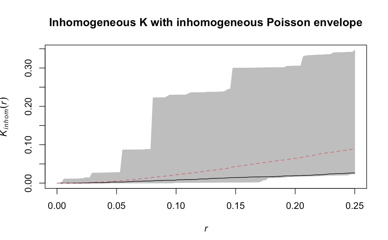
The observed inhomogeneous $K$ function lies entirely within the simulated inhomogeneous Poisson envelope, meaning that once spatial variation in intensity is accounted for, there is no evidence of significant clustering. The clustering seen in the homogeneous $K$ plot was likely caused by intensity gradients, not true point interactions.
6. Conclusion
Ripley’s $K$ and Besag’s $L$ function allow us to analyze how the spatial structure of a point pattern changes with distance. By examining $\hat{K}(r)$ or $\hat{L}(r)-r$ across a range of $r$, we can see whether points are clustered or just randomly distributed at different spatial scales.
Other Materials
Presentation Materials for SPH5105 Advanced Geospatial Methods for Public Health