Summary: This note explains variational inference (VI) as a scalable alternative to MCMC for approximate Bayesian inference. It introduces entropy, cross-entropy, and KL divergence, then contrasts forward (zero-avoiding) vs. reverse (zero-forcing) KL. The ELBO is derived as a tractable optimization target, enabling posterior approximation via Monte Carlo estimation, reparameterization, and mini-batching.

Introduction

In Bayesian statistics, statistical inference often poses significant computational challenges, particularly due to the complexity and intractability of posterior distributions. In practical applications, especially with large datasets and complex model structures such as microsimulation models or variational autoencoders (VAEs), the posterior distribution cannot be derived analytically. As a result, researchers frequently resort to approximate inference techniques rather than pursuing exact solutions.

Among these, Markov Chain Monte Carlo (MCMC) methods are widely used due to their theoretical soundness. However, MCMC can be computationally intensive, slow to converge, and difficult to scale to large datasets. To address these limitations, variational inference (VI) has emerged as an efficient alternative. Variational methods transform the inference problem into an optimization problem, offering computational advantages similar to maximum a posteriori (MAP) estimation while maintaining reasonable approximation accuracy. This makes VI particularly appealing for large-scale applications.

The core idea of variational inference is to approximate the true posterior distribution with a simpler, tractable distribution selected from a predefined family. To perform this approximation, one must first define a measure of similarity between the true posterior and the variational distribution—typically using the Kullback–Leibler (KL) divergence—as a criterion to guide the optimization.

Kullback-Leibler Divergence

In information theory, entropy is a fundamental concept used to quantify the average amount of information contained in a random variable $X$ with probability distribution $P$. It is defined as:

where the summation is taken over the support of $X$. Entropy represents the expected amount of information (or uncertainty) associated with outcomes drawn from the distribution $P$.

When we wish to measure the expected number of bits needed to encode samples from $P$ using a code optimized for a different distribution $Q$, we use cross-entropy, defined as:

Cross-entropy penalizes the mismatch between the true distribution $P$ and the candidate distribution $Q$.

To formally quantify the divergence between two distributions $P$ and $Q$, we use the concept of relative entropy, more commonly known as the Kullback–Leibler (KL) divergence, defined as:

where we can see KL-divergence is exactly the difference between entropy and cross entropy. ==In other words, the KL-divergence is the average extra amount of information required to encode the data using the candidate probability distribution instead of the actual distribution==.

We can easily extend the definition of continuous variable $X$ to the form:

where $P$ and $Q$ are probability distribution of the continuous random variable $X$ and $p$ and $q$ represent the probability density functions.

The KL-divergence is non-negative (Theorem 1.1 Gibbs’ Inequality), non-symmetric and is equal to $0$ or $\infty$ for two perfectly matching and non-matching distributions, respectively.

Evidence Lower Bound (ELBO)

Since the KL divergence quantifies the information discrepancy between two probability distributions, it can be used to evaluate how close an approximate distribution is to a target distribution. Specifically, in approximate Bayesian inference, instead of sampling directly from the exact posterior distribution as in Markov Chain Monte Carlo (MCMC), we can minimize the KL divergence between a parameterized proposal distribution $p(z)$ and the true posterior distribution $p(z|x)$. This provides a principled way to approximate the posterior by solving an optimization problem. However, due to the asymmetry of KL divergence, the direction in which the divergence is minimized must be carefully considered in the formulation of the inference method.

Forward vs. Reverse KL

First, consider the forward KL divergence (also called the M-projection). We aim to find

Because this objective requires taking an expectation under the true posterior $P(Z\mid X)$, it is generally intractable in practice. Moreover, the forward KL heavily penalizes any region where $q(x)$ assigns near-zero mass but the true density $p(x)$ is positive:

As a result, minimizing $D_{KL}(P|q)$ forces $q(x)$ to remain strictly positive wherever $p(x)>0$. This zero avoiding behavior ensures that $q$ covers the full support of $p$, often at the cost of over-estimating low-probability regions.

By contrast, the reverse KL divergence (or I-projection) is defined as

which only requires expectations under q and is therefore tractable when $\mathcal{Q}$ is chosen wisely. The reverse KL instead penalizes regions where $q(x)>0$ but $p(x)=0$, since

Minimizing $D_{KL}(q|P)$ thus drives $q(x)$ to zero wherever the true density vanishes—a zero forcing effect that makes $q$ concentrate on the modes of $p$, potentially ignoring its tails.

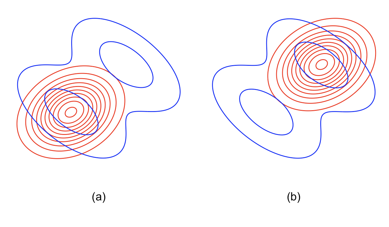
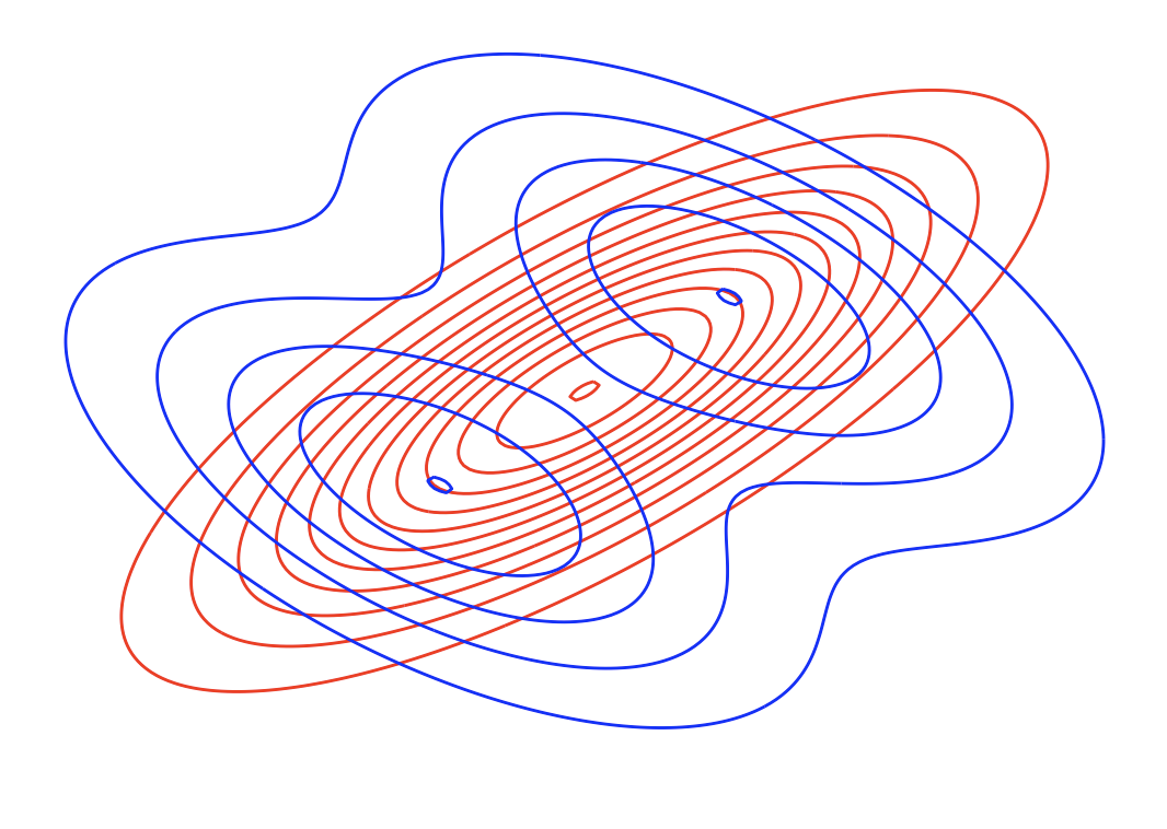
In practice, forward KL (zero-avoiding) tends to produce broader approximations that cover all of p’s support, whereas reverse KL (zero-forcing) yields more peaked approximations focused on the highest-density regions.

Formulation

Given the tractability of the reverse KL, we formulate the following optimization problem:

Target:

\[q^{*}(z \mid x, \theta) = \arg\min_{\theta} D_{\mathrm{KL}}(q(z \mid x, \theta)\, || \,p(z\|x,\phi))\]

However, the current expectation is still not tractable as it requires the computation of the posterior distribution $p(z\mid x,\phi)$. Hence,

According to $(1)$, we denote Evidence Lower BOund (ELBO) (Interpretation of Evidence Lower Bound (ELBO)) as:

Therefore, in $\mathcal{L}$, we further separate joint distribution $p(x,z|\phi)$:

In the last equation in $(2)$, While placing $p(x \mid z, \phi)$ in the denominator is mathematically valid, it is conceptually inappropriate, as the variational objective aims to approximate the posterior by aligning $q(z \mid x, \theta)$ with the prior—not the likelihood.

Now our target has become maximizing the ELBO:

Mostly in reality, we can’t compute the liklihood exactly in VAEs or Transformers, so we apply Monte Carlo estimation to get the unbiased approximation (Unbiasedness of Monte Carlo Integral):

This is often done with:

1. Re-parameterization trick
2. Mini-batches for scalable training

Appendix

Lemma 1.1 Jenson’s Inequality

Assume a convex function $f(x)$, $x\in \mathbb{R}^N$, with probability density function $p(x)$ defined on $\mathbb{R}^N$, we have

\[\mathbb{E}\left[f(X)\right]\geq f(\mathbb{E}\left[X\right])\]

Proof: Since $f(x)$ is a convex function, then from the definition of convex functions, we directly have $\forall x_1, x_2\in \mathbb{R}^N,t\in[0,1]$,

Then we expand the induction to multiple points using math induction technique: Assume we have $\sum_{i=1}^N\lambda_i=1,\lambda_i\in [0,1],i=1,\cdots,N$, and $x_i\in \mathbb{R}^N$, where $x_i \ne x_j, \text{for all } i \ne j$.

When $N = 1$, then $f(x_1)=f(x_1)$, the inequality holds. When $N = 2$, then it is just the definition of the convex function, the inequality still holds. Assume it still holds for $N=M$, $M»0$, so when $N=M+1$, we have $\sum_{i=1}^{M+1}\lambda_i=1$, then

Therefore, $\sum_{i=1}^N\lambda_if(x_i)\geq f(\sum_{i=1}^N\lambda_ix_i)$ holds for all $N>0$, which implies that the value of a convex combination of function evaluations is greater than or equal to the function evaluated at the convex combination of points. In other words, the function value over the convex hull is bounded above by the convex combination.

According to $(1)$, since $\sum_{i=1}^N\lambda_i=1$ and $\lambda_i\in[0,1]$ for $i=1,\cdots,N$, we can interpret the $\lambda_i$ as a discrete probability distribution. As $N\rightarrow \infty$, t> this naturally extends to a continuous distribution, where $\lambda_i$ corresponds to a probability density. In this case, the inequality $(1)$ becomes the expectation form of Jenson’s inequality:

Theorem 1.1 Gibbs’ Inequality

Let $p(x)$ and $q(x)$ be probability density functions defined over a common domain $\mathcal{X} \subset \mathbb{R}^{N}$, and suppose:

• $p(x)>0$ almost everywhere on $\mathcal{X}$,
• $q(x)>0$ wherever $p(x)>0$, and
• $\int_{\mathcal{X}}p(x)dx=\int_{\mathcal{X}}q(x)dx=1$

Then:

\[\int_{\mathcal{X}}p(x)\log\frac{p(x)}{q(x)}dx\geq 0\]

with equality holds if and only if $p(x)=q(x)$ almost everywhere on $\mathcal{X}$. This is also equivalent to saying $D_{KL}(p(x)||q(x))\geq 0$.

Proof: Recall that $-\log(x)$ is a strictly convex function. Therefore, we can apply Jenson’s Inequality, which says:

Hence,

Interpretation of Evidence Lower Bound (ELBO)

Since $\log p(x \mid \phi)$ is commonly referred to as the evidence, Equation (1) gives:

because the KL divergence is always non-negative proved by Gibbs’ Inequality. Therefore, $\mathcal{L}$ serves as a lower bound on the evidence, and is thus referred to as the Evidence Lower Bound (ELBO).

Unbiasedness of Monte Carlo Integral

Prove following Monte Carlo Integral is an unbiased estimation of the real liklihood function, where all $z^{(l)}$ are identically, independently sampled from $q(z)$

\[\mathbb{E}_{z\sim q}\left[\log(p(x|z,\phi)) \right]\approx\frac{1}{L}\sum_{l=1}^{L}\log p(x|z^{(l)}), \qquad z^{(l)}\sim q(z)\]

Proof: We directly take expectation of the form, e.g.

where the second equation holds because each $z^{(l)}$ are i.i.d samples.

References

Ganguly, A., & Earp, S. W. (2021). An introduction to variational inference. arXiv preprint arXiv:2108.13083.